本章中,我们将使用代码进行实践,通过对算法进行调优来构建性能良好的机器学习模型,并对模型的性能进行评估。
基于流水线的工作流 本节学习scikit-learn中的Pipeline类,它使得我们可以拟合出包含任意多个处理步骤的模型,并将模型用于新数据的预测。
加载威斯康辛乳腺癌数据集 首先获取乳腺癌数据集:
1
2
import pandas as pddf = pd.read_csv('http://archive.ics.uci.edu/ml/machine-learning-databases/breast-cancer-wisconsin/wdbc.data' , header=None )
该数据集划分为32列,前两列是样本唯一ID和对样本的诊断结果(M代表恶性,B代表良性),后面的几列是包含了30个从细胞核照片中提取的特征。接下来,将数据集的30个特征赋值给数组对象X,同时转换诊断结果为数字:
1
2
3
4
5
6
7
from sklearn.preprocessing import LabelEncoderX = df.loc[:, 2 :].values y = df.loc[:, 1 ].values le = LabelEncoder() y = le.fit_transform(y) le.transform(['M' , 'B' ]) >> array([1 , 0 ], dtype=int64)
此时良性肿瘤和恶性肿瘤分别被标记为类0和类1。接下来将数据集划分为训练数据集和测试数据集:
1
2
from sklearn.model_selection import train_test_splitX_train, X_test, y_train, y_test = train_test_split(X, y, test_size=0.2 , random_state=1 )
在流水线中集成数据转换及评估操作 接下来可以直接使用Pipeline将上述步骤串联起来:
1
2
3
4
5
6
7
8
9
10
from sklearn.preprocessing import StandardScalerfrom sklearn.decomposition import PCAfrom sklearn.linear_model import LogisticRegressionfrom sklearn.pipeline import Pipelinepipe_lr = Pipeline([('scl' , StandardScaler()), ('pca' , PCA(n_components=2 )), ('clf' , LogisticRegression(random_state=1 ))]) pipe_lr.fit(X_train, y_train) print (pipe_lr.score(X_test, y_test))>> 0.9473684210526315
Pipeline对象使用元组的序列作为输入,其中每个元组的第一个值为字符串,它可以是任意的标识符,我们通过它来访问流水线中的元素,而元组的第二个值为scikit-learn中的以恶转换器或者是评估器。
使用k折交叉验证评估模型性能 本节中,我们学习两种有用的交叉验证技术:holdout交叉验证 和k折交叉验证 。借助于这两种方法,我们可以得到模型泛化误差的可靠估计,即模型在新数据上的性能表现。
holdout方法 使用holdout进行模型选择更好的方法是将数据分为三个部分:训练数据集,验证数据集和测试数据集。训练数据集用于不同模型的拟合,模型在验证数据集上的性能表现作为模型选择的标准。使用模型训练和模型选择阶段不曾使用的数据作为测试数据集的优势在于:评估模型应用于新数据上能够获得较小偏差。
holdout方法的一个缺点是:模型性能的评估对训练数据集划分为训练及验证子集的方法是敏感的,评价的结果会随着样本的不同而发生变化。下一节介绍鲁棒性更好的性能评价技术:k折交叉验证,我们将在k个训练数据子集上重复holdout方法k次。
k折交叉验证 在k折交叉验证中,我们不重复地随机将训练数据集划分为k个,其中$ k-1 $个用于模型的训练,剩余的1个用于测试。重复此过程k次,我们就得到了k个模型及对模型性能的评价。
由于k折交叉验证使用了无重复抽样技术,该方法的优势在于每个样本点只有一次被划入训练数据集或者测试数据集的机会,与holdout方法相比,这将会使得模型性能的评估具有较小的方差。
留一(LOO)交叉验证:在LOO中,我们将数据子集划分的数量等同于样本数(k = n),这样每次只有一个样本用于测试。
分层k折交叉验证相对于k折交叉验证做了稍许改进,它可以得到更低的偏差或方差。接下来通过scikit-learn中的StratifiedKFold迭代器来演示:
1
2
3
4
5
6
7
8
9
10
11
import numpy as npfrom sklearn.model_selection import StratifiedKFoldkfold = StratifiedKFold(n_splits=10 , random_state=1 ) scores = [] k = 0 for train, test in kfold.split(X_train, y_train): pipe_lr.fit(X_train[train], y_train[train]) score = pipe_lr.score(X_train[test], y_train[test]) scores.append(score) k += 1 print ('Fold: %s, Class dist.: %s, Acc: %.3f' % (k, np.bincount(y_train[train]), score))
得到的结果如下:
1
2
3
4
5
6
7
8
9
10
Fold: 1 , Class dist.: [256 153 ], Acc: 0.891 Fold: 2 , Class dist.: [256 153 ], Acc: 0.978 Fold: 3 , Class dist.: [256 153 ], Acc: 0.978 Fold: 4 , Class dist.: [256 153 ], Acc: 0.913 Fold: 5 , Class dist.: [256 153 ], Acc: 0.935 Fold: 6 , Class dist.: [257 153 ], Acc: 0.978 Fold: 7 , Class dist.: [257 153 ], Acc: 0.933 Fold: 8 , Class dist.: [257 153 ], Acc: 0.956 Fold: 9 , Class dist.: [257 153 ], Acc: 0.978 Fold: 10 , Class dist.: [257 153 ], Acc: 0.956
尽管之前的代码清楚介绍了k折交叉验证的工作方式,scikit-learn同样实现了k折交叉验证评分的计算,这时的我们可以更加高效地使用分层k折交叉验证对模型进行评估:
1
2
3
4
5
6
from sklearn.model_selection import cross_val_scorescores = cross_val_score(estimator=pipe_lr, X=X_train, y=y_train, cv=10 , n_jobs=1 ) print (scores)>> [0.89130435 0.97826087 0.97826087 0.91304348 0.93478261 0.97777778 0.93333333 0.95555556 0.97777778 0.95555556 ] print ('CV Acc: %.3f +/- %.3f' % (np.mean(scores), np.std(scores)))>> CV Acc: 0.950 +/- 0.029
通过学习及验证曲线来调试算法 在本节中,我们将会学习两个有助于提高学习算法性能的简单但功能强大的判定工具:学习曲线 (learning curve)与验证曲线 (validation curve)。
使用学习曲线判定偏差和方差问题 通过将模型的训练及准确性验证看作是训练数据集大小的函数,并且绘制其图像,可以很容易地看出来模型面临高方差还是高偏差。
高偏差模型的训练准确率和交叉验证准确率都很低,这表明此模型未能很好地拟合数据。而高方差模型训练准确率和交叉验证准确率之间相差很大。
接下来,使用scikit-learn中的学习曲线函数评估模型:
1
2
3
4
5
6
7
8
9
10
11
12
13
14
15
16
17
18
19
20
21
22
23
24
import matplotlib.pyplot as pltfrom sklearn.model_selection import learning_curvepipe_lr = Pipeline([('scl' , StandardScaler()), ('clf' , LogisticRegression(penalty='l2' , random_state=0 ))]) train_sizes, train_scores, test_scores = learning_curve(estimator=pipe_lr, X=X_train, y=y_train, train_sizes=np.linspace(0.1 , 1.0 , 10 ), cv=10 , n_jobs=1 ) train_mean = np.mean(train_scores, axis=1 ) train_std = np.std(train_scores, axis=1 ) test_mean = np.mean(test_scores, axis=1 ) test_std = np.std(test_scores, axis=1 ) plt.plot(train_sizes, train_mean, color='b' , marker='o' , label='training acc.' ) plt.fill_between(train_sizes, train_mean + train_std, train_mean - train_std, alpha=0.15 , color='b' ) plt.plot(train_sizes, test_mean, color='r' , marker='s' , label='validation acc' ) plt.fill_between(train_sizes, test_mean + test_std, test_mean - test_std, alpha=0.15 , color='r' ) plt.grid() plt.xlabel('Number of training samples' ) plt.ylabel('Accuracy' ) plt.legend() plt.ylim([0.8 , 1.0 ]) plt.show()
可以得到如下图像:
从图像可知,模型在测试数据集上表现良好。
通过验证曲线来判定过拟合和欠拟合 验证曲线和学习曲线类似,不过绘制的不是样本大小和训练准确率,测试准确率之间的关系,而是准确率与模型参数之间的关系,例如逻辑斯蒂回归模型中的正则化参数倒数C。下面使用scikit-learn来绘制验证曲线:
1
2
3
4
5
6
7
8
9
10
11
12
13
14
15
16
17
18
19
20
21
22
23
from sklearn.model_selection import validation_curveparam_range = [0.001 , 0.01 , 0.1 , 1.0 , 10.0 , 100.0 ] train_scores, test_scores = validation_curve(estimator=pipe_lr, X=X_train, y=y_train, param_name='clf__C' , param_range=param_range, cv=10 ) train_mean = np.mean(train_scores, axis=1 ) train_std = np.std(train_scores, axis=1 ) test_mean = np.mean(test_scores, axis=1 ) test_std = np.std(test_scores, axis=1 ) plt.plot(param_range, train_mean, color='b' , marker='o' , label='training acc.' ) plt.fill_between(param_range, train_mean + train_std, train_mean - train_std, alpha=0.5 , color='b' ) plt.plot(param_range, test_mean, color='r' , marker='s' , label='validation acc.' ) plt.fill_between(param_range, test_mean + test_std, test_mean - test_std, alpha=0.5 , color='b' ) plt.grid() plt.xscale('log' ) plt.legend() plt.xlabel('Parameter C' ) plt.ylabel('Acc.' ) plt.ylim([0.8 , 1.0 ]) plt.show()
得到的图像如下:
在本例中,需要验证的是参数C,即定义在scikit-learn流水线中的逻辑斯蒂回归分类器的正则化参数,我们将其记为clf__C,并且通过param_range参数来设定其值的范围。
从上图可以看到,如果加大正则化强度(较小的C值),会导致模型的欠拟合;如果增加C的值,模型又会趋向于过拟合,在本例中,最优点在$ C=0.1 $附近。
使用网格搜索调优机器学习模型 机器学习中,有两类参数:通过训练数据学习得到的参数,如逻辑斯蒂回归中的回归系数;以及学习算法中需要单独进行优化的参数。后者是调优参数,也称为超参,对模型来说,就如逻辑斯蒂回归中的正则化系数,或者决策树中的深度参数。
接下来,我们学习一种更加强大的超参数优化技巧:网格搜索 (grid search),它通过寻找最优的超参数值的组合以进一步提高模型的性能。
使用网络搜索调优参数 网格搜索法很简单,它通过对我们指定的不同超参列表进行暴力穷举法,来计算评估每个组合对模型性能的影响,以获得参数的最优组合:
1
2
3
4
5
6
7
8
9
10
11
from sklearn.model_selection import GridSearchCVfrom sklearn.svm import SVCpipe_svc = Pipeline([('scl' , StandardScaler()), ('clf' , SVC(random_state=1 ))]) param_range = [0.0001 , 0.001 , 0.01 , 0.1 , 1.0 , 10.0 , 100.0 , 1000.0 ] param_grid = [{'clf__C' : param_range, 'clf__kernel' : ['linear' ]}, {'clf__C' : param_range, 'clf__gamma' : param_range, 'clf__kernel' : ['rbf' ]}] gs = GridSearchCV(estimator=pipe_svc, param_grid=param_grid, scoring='accuracy' , cv=10 , n_jobs=-1 ) gs.fit(X_train, y_train) print (gs.best_score_, gs.best_params_)>> 0.978021978021978 {'clf__C' : 0.1 , 'clf__kernel' : 'linear' }
在本例中,线性SVM模型可得到的最优k折交叉验证准确率为$ 97.8% $。
最后,我们使用独立的测试数据集,通过GridSearchCV对象的best_estimator_属性对最优模型进行评估:
1
2
3
4
clf = gs.best_estimator_ clf.fit(X_train, y_train) print (clf.score(X_test, y_test))>> 0.9649122807017544
虽然网格搜索时寻找最优参数集合的一种功能强大的方法,但是他的计算成本时很高的,此时可以尝试使用另外一种方法:随即搜索(randomized search)。该方法在scikit-learn中的RandomizedSearchCV类已经实现。
通过嵌套交叉验证选择算法 上一节的方法由于在同一个算法中找到最优超参,而本节中介绍的方法用于在不同的机器学习算法中找到最优的机器算法,它就是嵌套交叉验证。
在嵌套交叉验证中,我们将数据划分为训练块和测试块;而在用于模型选择的内部循环中,我们则基于这些训练块使用k折交叉验证。在完成模型的选择后,测试块用于模型性能的评估。
借助于scikit-learn,我们可以通过如下方法使用嵌套交叉验证:
1
2
3
4
gs = GridSearchCV(estimator=pipe_svc, param_grid=param_grid, scoring='accuracy' , cv=10 , n_jobs=-1 ) scores = cross_val_score(gs, X, y, scoring='accuracy' , cv=5 ) print ('CV acc: %.3f +/- %.3f' % (np.mean(scores), np.std(scores)))>> CV acc: 0.972 +/- 0.012
代码返回的交叉验证准确率平均值对模型超参调优的预期值给出了很好的估计,且使用该值优化过的模型呢能够预测未知数据。例如,我们可以使用嵌套交叉验证方法比较SVM模型与决策树分类器;为了简单起见,我们只调优数的深度参数:
1
2
3
4
5
6
7
8
from sklearn.tree import DecisionTreeClassifiergs = GridSearchCV(estimator=DecisionTreeClassifier(random_state=0 ), param_grid=[{'max_depth' : [1 , 2 , 3 , 4 , 5 , 6 , 7 , None ]}], scoring='accuracy' , cv=5 ) scores = cross_val_score(gs, X_train, y_train, scoring='accuracy' , cv=5 ) print ('CV acc: %.3f +/- %.3f' % (np.mean(scores), np.std(scores)))>> CV acc: 0.908 +/- 0.045
从两个算法的输出看,嵌套交叉验证对SVM的评价高于决策树。由此可见,SVM是用于对测数据集未知数据进行分类的一个更好的选择。
了解不同的性能评价指标 前面的几个章节中,我们使用的都是模型准确性来对模型进行评估,接下来学习其他几个性能指标:准确率 (precision),召回率 (recall),F1分数 (F1-score)。
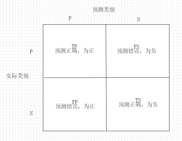
读取混淆矩阵 首先,了解一下混淆矩阵:
虽然这些指标可以人工比较的到结果,但是scikit-learn提供了一个confusion_matrix函数:
1
2
3
4
5
6
7
from sklearn.metrics import confusion_matrixpipe_svc.fit(X_train, y_train) y_pred = pipe_svc.predict(X_test) conmat = confusion_matrix(y_true=y_test, y_pred=y_pred) print (conmat)>> [[71 1 ] >> [ 2 40 ]]
在执行上述代码后,我们可以得到混淆矩阵。在本例中,假定类别1是正类,模型正确预测了71个属于类别0的样本(真负),以及40个属于类别1的样本(真正)。
优化分类模型的准确率和召回率 预测准确率(ACC)和预测误差率(ERR)都提供了样本分类的相关信息。他们的计算方法如下:
1
2
3
4
5
6
7
8
from sklearn.metrics import precision_scorefrom sklearn.metrics import recall_score, f1_scoreprint ('Pre.: %.3f' % precision_score(y_true=y_test, y_pred=y_pred))print ('Rec.: %.3f' % recall_score(y_true=y_test, y_pred=y_pred))print ('F1.: %.3f' % f1_score(y_true=y_test, y_pred=y_pred))>> Pre.: 0.976 >> Rec.: 0.952 >> F1.: 0.964
请记住scikit-learn中将正类类标标识为1 。如果我们想要指定一个不同的类标,可以通过make_scorer来构建我们自己的评分,这样我们可以将其应用于GridSearchCV:
1
2
3
from sklearn.metrics import make_scorer, f1_scorescorer = make_scorer(f1_score, pos_label=0 ) gs = GridSearchCV(estimator=pipe_svc, param_grid=param_grid, scoring=scorer, cv=10 )
ROC曲线 受试者工作特征曲线 (receiver operator characteristic,ROC)是基于假正率和真正率等性能指标进行分类模型选择的有用工具,假正率和真正率通过移动分类器的阈值实现。基于ROC曲线,我们可以计算所谓的ROC线下区域(AUC),用来刻画分类模型的性能。
在scikit-learn中ROC AUC得分可以通过roc_auc_score函数计算得到:
1
2
3
4
5
from sklearn.metrics import roc_auc_score, accuracy_scoreprint ("ACC: %.3f" % (accuracy_score(y_true=y_test, y_pred=y_pred)))print ('ROC AUC: %.3f' % (roc_auc_score(y_true=y_test, y_score=y_pred)))>> ACC: 0.974 >> ROC AUC: 0.969
通过ROC AUC得到的分类器性能可以让我们进一步洞悉分类器在类别不均衡样本集合上的性能。
多类别分类的评价标准 本节中讨论的评分标准都是基于二分类系统的。不同,scikit-learn实现了macro(宏)和micro(微)均值方法,计算公式如下: