本章中,我们将会学习如何构建一组分类器的集合,使得整体分类效果优于其中任意一个单独的分类器。
集成学习 集成方法 (ensemble method)的目标是:将不同的分类器组合成一个元分类器,与包含于其中的单个分类器相比,元分类器具有更好的泛化性能。
本章中介绍的几种流行的集成方法,它们都使用了多数投票 (majority voting)。多数投票原则是将大多数分类器预测的结果作为最终的预测指标。基于训练集,我们首先训练m个不同的成员分类器($ C_1, \cdots, C_m $),接着我们将新的未知数据$ x $输入,然后对所有分类器$ C_j $的预测类标进行汇总,选择出得票率最高的类标$ \hat{y} $:
mode函数:众数函数,返回出现次数最多的值。
另外,由统计学知识得到,当成员分类器出错率低于$ 50% $时,集成分类器的出错率要低于单个分类器。
实现一个简单的多数投票分类器 集成算法允许我们使用单独的权重对不同分类算法进行组合,可以将加权多数投票记为:
argmax是一种函数,是对函数求参数(集合)的函数。当我们有另一个函数$ y=f(x) $时,若有结果$ x_0= argmax(f(x)) $,则表示当函数$ argmax(f(x)) $取$ x=x_0 $的时候,得到f(x)取值范围的最大值;若有多个点使得f(x)取得相同的最大值,那么$ argmax(f(x)) $的结果就是一个点集。
为了使用Python代码实现加权多数投票,我们可以使用NumPy中的argmax和bincount函数:
1
2
3
import numpy as npnp.argmax(np.bincount([0 , 0 , 1 ], weights=[0.2 , 0.2 , 0.6 ])) >> 1
在实际应用中,我们可以将原来的类标转换为预测类表的概率,这样修正公式如下:
为实现基于类别预测概率的加权多数投票,我们可以使用如下代码:
1
2
3
4
5
6
ex = np.array([[0.9 , 0.1 ], [0.8 , 0.2 ], [0.4 , 0.6 ]]) p = np.average(ex, axis=0 , weights=[0.2 , 0.2 , 0.6 ]) print (p, np.argmax(p))>> [0.58 0.42 ] 0
综上,我们可以实现MajorityVoteClassifier:
1
2
3
4
5
6
7
8
9
10
11
12
13
14
15
16
17
18
19
20
21
22
23
24
25
from sklearn.base import BaseEstimatorfrom sklearn.base import ClassifierMixinfrom sklearn.preprocessing import LabelEncoderfrom sklearn.externals import sixfrom sklearn.base import clonefrom sklearn.pipeline import _name_estimatorsimport numpy as npimport operatorclass MajorityVoteClassifier (BaseEstimator, ClassifierMixin): def __init__ (self, classifiers, vote='classlabel' , weights=None ): self.classifiers = classifiers self.named_classifiers = {key: value for key, value in _name_estimators(classifiers)} self.vote = vote self.weights = weights def fit (self, X, y ): self.labelenc_ = LabelEncoder() self.labelenc_.fit(y) self.classes_ = self.labelenc_.classes_ self.classifiers_ = [] for clf in self.classifiers: fitted_clf = clone(clf).fit(X, self.labelenc_.transform(y)) self.classifiers_.append(fitted_clf) return self
在这里,我们使用了两个基类BaseEstimator和ClassifierMixIn获取某些基本方法,包括设定分类器参数的set_params和返回参数的get_params方法,以及用于计算预测准确度的score方法。此外,导入six包是为了使得MajorityVoteClassifier与Python 2.7兼容。
接下来,我们加入predict方法:
1
2
3
4
5
6
7
8
9
10
11
12
13
14
15
16
17
18
19
20
21
22
23
24
25
26
def predict (self, X ): if self.vote == 'probability' : maj_vote = np.argmax(self.predict_proba(X), axis=1 ) else : predictions = np.asarray([clf.predict(X) for clf in self.classifiers_]).T maj_vote = np.apply_along_axis(lambda x: np.argmax(np.bincount(x, weights=self.weights)), axis=1 , arr=predictions) maj_vote = self.labelenc_.inverse_transform(maj_vote) return maj_vote def predict_proba (self, X ): probas = np.asarray([clf.predict_proba(X) for clf in self.classifiers_]) avg_proba = np.average(probas, axis=0 , weights=self.weights) return avg_proba def get_params (self, deep=True ): if not deep: return super (MajorityVoteClassifier, self).get_params(deep=False ) else : out = self.named_classifiers.copy() for name, step in six.iteritems(self.named_classifiers): for key, value in six.iteritems(step.get_params(deep=True )): out['%s__%s' % (name, key)] = value return out
接下来我们可以将上述算法用于实战了。我们导入鸢尾花数据集,并且只是用其中的两个特征:萼片宽度 和花瓣长度 。同时我们只区分两个类别的样本:Iris-Versicolor和Iris-Virginica,并且绘制ROC AUC曲线:
1
2
3
4
5
6
7
8
9
from sklearn import datasetsfrom sklearn.model_selection import train_test_splitfrom sklearn.preprocessing import StandardScalerfrom sklearn.preprocessing import LabelEncoderiris = datasets.load_iris() X, y = iris.data[50 :, [1 , 2 ]], iris.target[50 :] le = LabelEncoder() y = le.fit_transform(y)
下面划分数据集为测试数据集和训练数据集:
1 X_train, X_test, y_train, y_test = train_test_split(X, y, test_size=0.5 , random_state=1 )
接下来将数据集训练三种不同类型的分类器:逻辑斯蒂回归分类器,决策树分类器和k-近邻分类器各一个:
1
2
3
4
5
6
7
8
9
10
11
12
13
14
15
16
17
18
19
from sklearn.model_selection import cross_val_scorefrom sklearn.linear_model import LogisticRegressionfrom sklearn.tree import DecisionTreeClassifierfrom sklearn.neighbors import KNeighborsClassifierfrom sklearn.pipeline import Pipelineimport numpy as pyclf1 = LogisticRegression(penalty='l2' , C=0.01 , random_state=0 ) clf2 = DecisionTreeClassifier(max_depth=1 , criterion='entropy' , random_state=0 ) clf3 = KNeighborsClassifier(n_neighbors=1 , p=2 , metric='minkowski' ) pipe1 = Pipeline([['sc' , StandardScaler()], ['clf' , clf1]]) pipe3 = Pipeline([['sc' , StandardScaler()], ['clf' , clf3]]) clf_labels = ['LR' , 'DT' , 'KNN' ] for clf, label in zip ([pipe1, clf2, pipe3], clf_labels): scores = cross_val_score(estimator=clf, X=X_train, y=y_train, cv=10 , scoring='roc_auc' ) print ('ROC AUC: %.3f +/- %.3f [%s]' % (scores.mean(), scores.std(), label)) >> ROC AUC: 0.917 +/- 0.201 [LR] >> ROC AUC: 0.917 +/- 0.154 [DT] >> ROC AUC: 0.933 +/- 0.104 [KNN]
在此,为什么将逻辑斯蒂回归和k-近邻分类器的训练作为流水线的一部分?不同于决策树,逻辑斯蒂回归和k-近邻算法对数据缩放不敏感,需要对其进行数据标准化处理。
接下来我们基于多数投票原则,在其中组合成员分类器:
1
2
3
4
5
6
7
8
9
10
mv_clf = MajorityVoteClassifier(classifiers=[pipe1, clf2, pipe3]) clf_labels += ['MV' ] all_clf = (pipe1, clf2, pipe3, mv_clf) for clf, label in zip (all_clf, clf_labels): scores = cross_val_score(estimator=clf, X=X_train, y=y_train, cv=10 , scoring='roc_auc' ) print ('ROC AUC: %.3f +/- %.3f [%s]' % (scores.mean(), scores.std(), label)) >> ROC AUC: 0.917 +/- 0.201 [LR] >> ROC AUC: 0.917 +/- 0.154 [DT] >> ROC AUC: 0.933 +/- 0.104 [KNN] >> ROC AUC: 0.967 +/- 0.100 [MV]
从上述输出来看,以10折交叉验证作为评估标准,MajorityVotingClassifier的性能与单个成员分类器相比有着质的提高。
评估与调优集成分类器 接下来,我们将在测试数据上计算多数投票的ROC曲线,以验证其在未知数据上的泛化性能:
1
2
3
4
5
6
7
8
9
10
11
12
13
14
15
16
17
18
from sklearn.metrics import roc_curvefrom sklearn.metrics import aucfrom matplotlib import pyplot as pltcolors = ['black' , 'orange' , 'blue' , 'green' ] linestyles = [':' , '--' , '-.' , '-' ] for clf, label, clr, ls in zip (all_clf, clf_labels, colors, linestyles): y_pred = clf.fit(X_train, y_train).predict_proba(X_test)[:, 1 ] fpr, tpr, thresholds = roc_curve(y_true=y_test, y_score=y_pred) roc_auc = auc(x=fpr, y=tpr) plt.plot(fpr, tpr, color=clr, linestyle=ls, label='%s (auc = %.3f)' % (label, roc_auc)) plt.legend() plt.xlim([-0.1 , 1.1 ]) plt.ylim([-0.1 , 1.1 ]) plt.grid() plt.xlabel('False Positive Rate' ) plt.ylabel('True Postive Rate' ) plt.show()
得到的图像如下:
由ROC结果我们可以得到,继承分类器在测试集上表现优秀(ROC AUC = 0.95),而KNN分类器对于训练数据有些过拟合。
在学习集成分类的成员分类器调优之前,我们调用一下get_param方法:
输出如下:
1 2 3 4 5 6 7 8 9 10 11 12 13 14 15 16 17 18 19 {'pipeline-1' : Pipeline(memory=None , steps=[('sc' , StandardScaler(copy=True , with_mean=True , with_std=True )), ['clf' , LogisticRegression(C=0.01 , class_weight=None , dual=False , fit_intercept=True , intercept_scaling=1 , l1_ratio=None , max_iter=100 , multi_class='warn' , n_jobs=None , penalty='l2' , random_state=0 , solver='warn' , tol=0.0001 , verbose=0 , warm_start=False )]], verbose=False ), ... 'pipeline-2__clf__leaf_size' : 30 , 'pipeline-2__clf__metric' : 'minkowski' , 'pipeline-2__clf__metric_params' : None , 'pipeline-2__clf__n_jobs' : None , 'pipeline-2__clf__n_neighbors' : 1 , 'pipeline-2__clf__p' : 2 , 'pipeline-2__clf__weights' : 'uniform' }
接下来我们先通过网格搜索来调整逻辑斯蒂回归分类器的正则化系数倒数C以及决策深度:
1
2
3
4
5
6
7
8
from sklearn.model_selection import GridSearchCVparams = {'decisiontreeclassifier__max_depth' : [1 , 2 ], 'pipeline-1__clf__C' : [0.001 , 0.1 , 100.0 ]} grid = GridSearchCV(estimator=mv_clf, param_grid=params, cv=10 , scoring='roc_auc' ) grid.fit(X_train, y_train) res = grid.cv_results_ for params, mean_score, std_score in zip (res['params' ], res['mean_test_score' ], res['std_test_score' ]): print ('%.3f +/- %.3f %r' % (mean_score, std_score, params))
得到的结果如下:
1
2
3
4
5
6
0.967 +/- 0.100 {'decisiontreeclassifier__max_depth' : 1 , 'pipeline-1__clf__C' : 0.001 }0.967 +/- 0.100 {'decisiontreeclassifier__max_depth' : 1 , 'pipeline-1__clf__C' : 0.1 }1.000 +/- 0.000 {'decisiontreeclassifier__max_depth' : 1 , 'pipeline-1__clf__C' : 100.0 }0.967 +/- 0.100 {'decisiontreeclassifier__max_depth' : 2 , 'pipeline-1__clf__C' : 0.001 }0.967 +/- 0.100 {'decisiontreeclassifier__max_depth' : 2 , 'pipeline-1__clf__C' : 0.1 }1.000 +/- 0.000 {'decisiontreeclassifier__max_depth' : 2 , 'pipeline-1__clf__C' : 100.0 }
最优的参数和准确度如下:
1
2
3
print ('Best params: %s\nAcc: %.3f' % (grid.best_score_, grid.best_score_))>> Best params: 1.0 >> Acc: 1.000
可以发现,当选择正则化强度较小时,我们能得到最佳的交叉验证结果,而决策树的深度似乎没有什么影响。注意在模型评估时,不止一次使用测试集并非一个好的做法。接下来将学习另外一种集成方法:bagging。
在本节中我们实现的多数投票方法有时也成为堆叠(stocking)。
bagging–通过bootstrap样本构建集成分类器 bagging是一种与上节实现的MajorityVoteClassifier关系紧密的集成学习技术,但是不同的是这个算法没有使用相同的训练数据集拟合集成分类器中的单个成员分类器。由于原始数据集使用了bootstrap抽样(有放回的随机抽样),这也是bagging被称为bootstrap aggregating的原因。
接下来为了检验bagging的实际效果,我们用葡萄酒数据集构建一个更复杂的分类问题,在此我们只考虑葡萄酒中的类别2和类别3,且只选择Alcohol和Hue这两个特征:
1
2
3
4
5
6
7
8
9
10
11
12
import pandas as pddf_wine = pd.read_csv('./wine.data' , header=None ) df_wine.columns = ['Class label' , 'Alcohol' , 'Malic acid' , 'Ash' , 'Alcalinity' , 'Magnesium' , 'Total phenols' , 'Flavanoids' , 'Nonflavanoids' , 'Proanthocyanins' , 'Color intensity' , 'Hue' , 'Diluted' , 'Proline' ] df_wine = df_wine[df_wine['Class label' ] != 1 ] y = df_wine['Class label' ].values X = df_wine[['Alcohol' , 'Hue' ]].values
接下来,对类标进行编码,同时将数据集划分为测试集和训练集:
1
2
3
4
5
6
from sklearn.preprocessing import LabelEncoderfrom sklearn.model_selection import train_test_splitle = LabelEncoder() y = le.fit_transform(y) X_train, X_test, y_train, y_test = train_test_split(X, y, test_size=0.4 , random_state=1 )
scikit-learn中已经实现了Bagging Classifier相关算法,我们可以从ensemble子模块中导入使用:
1
2
3
4
5
6
7
8
9
10
11
from sklearn.ensemble import BaggingClassifiertree = DecisionTreeClassifier(criterion='entropy' , max_depth=None ) bag = BaggingClassifier(base_estimator=tree, n_estimators=500 , max_samples=1.0 , max_features=1.0 , bootstrap=True , bootstrap_features=False , n_jobs=-1 , random_state=1 )
接下来我们将计算训练数据集和测试数据集上的预测准确率:
1
2
3
4
5
6
7
8
9
from sklearn.metrics import accuracy_scoretree = tree.fit(X_train, y_train) y_train_pred = tree.predict(X_train) y_test_pred = tree.predict(X_test) tree_train = accuracy_score(y_train, y_train_pred) tree_test = accuracy_score(y_test, y_test_pred) print (tree_train, tree_test)>> 1.0 0.8333333333333334
基于上述代码执行的结果可见,未经剪枝的决策树显现出过拟合的现象。接下来看一下bag的拟合效果:
1
2
3
4
5
6
7
bag = bag.fit(X_train, y_train) y_train_pred = bag.predict(X_train) y_test_pred = bag.predict(X_test) bag_train = accuracy_score(y_train, y_train_pred) bag_test = accuracy_score(y_test, y_test_pred) print (tree_train, tree_test)>> 1.0 0.8958333333333334
从上图可见bagging分类器在测试数据上的泛化性能稍有胜出。接下来看一下它们的决策区域:
1
2
3
4
5
6
7
8
9
10
11
12
13
14
15
16
x_min = X_train[:, 0 ].min () - 1 x_max = X_train[:, 0 ].max () + 1 y_min = X_train[:, 1 ].min () - 1 y_max = X_train[:, 1 ].max () + 1 xx, yy = np.meshgrid(np.arange(x_min, x_max, 0.1 ), np.arange(y_min, y_max, 0.1 )) f, axarr = plt.subplots(nrows=1 , ncols=2 , sharex='col' , sharey='row' , figsize=(8 , 3 )) for idx, clf, tt in zip ([0 , 1 ], [tree, bag], ['DT' , 'Bagging' ]): clf.fit(X_train, y_train) Z = clf.predict(np.c_[xx.ravel(), yy.ravel()]) Z = Z.reshape(xx.shape) axarr[idx].contourf(xx, yy, Z, alpha=0.3 ) axarr[idx].scatter(X_train[y_train==0 , 0 ], X_train[y_train==0 , 1 ], c='b' , marker='^' ) axarr[idx].scatter(X_train[y_train==1 , 0 ], X_train[y_train==1 , 1 ], c='r' , marker='o' ) axarr[idx].set_title(tt) axarr[0 ].set_ylabel('Alcohol' ) plt.show()
可以得到图像如下:
从结果可见,和深度为3的决策树相比,bagging集成分类器的决策边界显得更加平滑。
bagging算法是降低模型方差的一种有效方法,但是它在降低模型偏差方面的作用不大。
通过自适应boosting提高弱学习机的性能 在本节中,重点讨论boosting算法的一个常用例子:Adaboost (Adaptive Boosting)。
在boosting中,集成分类器包含多个非常简单的成原分类器,这些成原分类器的性能仅仅好于随即猜测,常被称为弱学习机。原始的boosting过程如下:
从训练集D中以无放回抽样方式随机抽取一个训练子集$ d_1 $,用于弱学习机$ C_1 $的训练
从D中无放回抽样抽取一个训练子集$ d_2 $,并且将$ C_1 $中误分类样本的50%加入到训练集中,训练得到弱学习机$ C_2 $
从训练集中抽取$ C_1 $和$ C_2 $分类结果不一致的样本生成训练样本$ d_3 $,以此训练第三个弱学习机$ C_3 $
通过多数投票组合三个弱学习机$ C_1,C_2,C_3 $
和bagging模型相比,boosting可以同时降低偏差和方差。在实践中,boosting算法对训练数据有过拟合的倾向。
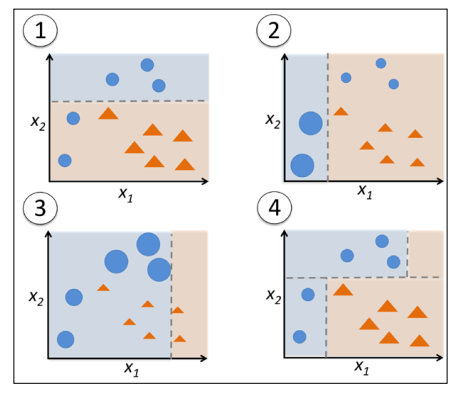
Adaboost和原始的boosting算法不同,它使用整个训练集来训练弱学习机,其中训练样本在每次迭代中都会重新被赋予一个权重,在上一弱学习机错误的基础上进行学习从而构建一个更加强大的分类器。
如上图,从图1开始,所有的样本都被赋予相同的权重,基于次训练集,我们得到了一个分类器(决策曲线是图中虚线);在下一轮中,我们为前面误分类的样本赋予更高的权重,此外我们降低被正确分类的样本的权重,如子图2所示,弱学习机错误划分了圆形类的三个样本,它们将在子图3中被赋予更大的权重…重复以上过程,最终组合三个学习机得到新的决策区域如图4。
下面是AdaBoost算法的基本步骤:
以等值的方式为权重向量$ w $赋值,其中$ \sum_iw_i=1 $
在m轮boosting操作中,对第j轮做如下操作
训练一个加权的弱学习机:$ C_j = train(X, y, w) $
预测样本类标:$ \hat{y} = =predict(C_j, X) $
计算权重错误率:$ \epsilon = w \cdot (\hat{y} == y)$
计算相关系数:$ a_j = 0.5log\frac{1-\epsilon} {\epsilon}$
更新权重:$ w = w \times exp(-a_j\times \hat{y} \times y) $
归一化权重:$ w:=w/\sum_i{w_i} $
完成最终预测:$ \hat{y} = (\sum_{j=1}^{m}(a_j\times predict(C_j, X)) > 0) $
下面通过scikit-learn来训练一个AdaBoost集成分类器,我们仍然使用上一节中的葡萄酒数据集:
1
2
3
4
5
6
7
8
9
10
from sklearn.ensemble import AdaBoostClassifiertree = DecisionTreeClassifier(criterion='entropy' , max_depth=1 ) ada = AdaBoostClassifier(base_estimator=tree, n_estimators=500 , learning_rate=0.1 , random_state=0 ) tree = tree.fit(X_train, y_train) y_train_pred = tree.predict(X_train) y_test_pred = tree.predict(X_test) tree_train = accuracy_score(y_train, y_train_pred) tree_test = accuracy_score(y_test, y_test_pred) print (tree_train, tree_test)>> 0.8450704225352113 0.8541666666666666
和上一节中未剪枝决策树相比,单层决策树对于训练数据过拟合的成都更加严重一点,接下来看一下AdaBoost分类器的性能:
1
2
3
4
5
6
7
ada = ada.fit(X_train, y_train) y_train_pred = ada.predict(X_train) y_test_pred = ada.predict(X_test) ada_train = accuracy_score(y_train, y_train_pred) ada_test = accuracy_score(y_test, y_test_pred) print (ada_train, ada_test)>> 1.0 0.875
可以发现,A大Boost模型准确预测了所有的训练集类标,与单层决策树相比,它在测试集上的表现良好,不过,在代码中也可以看到,我们在降低模型偏差的同时使得方差额外的增加。
最后看一下决策区域的形状:
1
2
3
4
5
6
7
8
9
10
11
12
13
14
15
16
x_min = X_train[:, 0 ].min () - 1 x_max = X_train[:, 0 ].max () + 1 y_min = X_train[:, 1 ].min () - 1 y_max = X_train[:, 1 ].max () + 1 xx, yy = np.meshgrid(np.arange(x_min, x_max, 0.1 ), np.arange(y_min, y_max, 0.1 )) f, axarr = plt.subplots(nrows=1 , ncols=2 , sharex='col' , sharey='row' , figsize=(8 , 3 )) for idx, clf, tt in zip ([0 , 1 ], [tree, ada], ['DT' , 'AdaBoost' ]): clf.fit(X_train, y_train) Z = clf.predict(np.c_[xx.ravel(), yy.ravel()]) Z = Z.reshape(xx.shape) axarr[idx].contourf(xx, yy, Z, alpha=0.5 ) axarr[idx].scatter(X_train[y_train==0 , 0 ], X_train[y_train==0 , 1 ], c='b' , marker='^' ) axarr[idx].scatter(X_train[y_train==1 , 0 ], X_train[y_train==1 , 1 ], c='r' , marker='o' ) axarr[idx].set_title(tt) axarr[0 ].set_ylabel('Alcohol' ) plt.show()
得到的图像如下:
从上图可知,AdaBoost的决策区域比单层决策树的决策区域复杂得多。